Seismo Blog
The seismic signals (ground vibrations) generated by the motion of the Oso landslide were very well recorded by the Pacific Northwest Seismic Network (PNSN), indicating it was a very rapid and energetic event (though this is apparent from the tragic consequences and eyewitness reports). Signals at the lowest frequencies (long periods), which travel farthest before attenuating, have been detected up to ~274 km (~170 miles) away from the landslide (station DAVN) though this distance may increase as more data are analyzed.
Recordings from seismic stations that recorded the event well can be used to determine the timing of the sequence of events (see Timeline section and Figures 2-3). Seismic signals from landsliding are distinguished from other noise such as vibrations of distant earthquakes and human and natural noise local to the seismic station by the frequency content, duration, shape and other characteristics of the waveforms.
Background
Seismic signals from landslides are distinct from those generated by earthquakes (Figure 1). Energy is generally concentrated at lower frequencies (<5Hz) and the signal emerges gradually from the noise. Earthquake signals, on the other hand, have a broader range of frequency content and arrive suddenly with the sharp onset of P waves followed by often distinct S wave and surface wave arrivals. These distinct arrivals are typically not observable in landslide seismograms. The reason for the differences are different physical mechanisms that generate the waves. Earthquakes are generated by brittle slip along a fault plane deep in the earth that starts suddenly and lasts a very short time whereas landslides typically last several minutes or longer and energy builds up more slowly as the material accelerates and begins to break apart. The peak seismic amplitudes will be reached often toward the middle of the signal, peaking, and then gradually fading back into the noise again.
Not all landslides generate strong seismic signals observable at large distances. The event must be large and energetic for the resulting seismic waves to be observable tens to hundreds of km away. Most if not all of the Oso landslide subevents that were recorded seismically were probably generated by material breaking off the source area and moving rapidly downslope, not by slow creep or mud moving slowly in the valley.

Figure 1: Comparison between seismic signals characteristic of A.) a regular small earthquake signal (this is the M1.1 that occured on March 10th near the Oso slide) and B.) a landslide (this is the first slide from the Oso sequence). Note the x-axis is of equal duration in both cases. Click to enlarge.

Figure 2: Google Earth map of landslide location relative to seismic stations referred to in this report.
Timeline
The seismic data recorded at the closest station, Jim Creek Washington (JCW, Figure 2), is displayed in webicorder format on Figure 3. This figure can be read like a book, each line shows 30 minutes of conitnuous seismic data collected at 100 samples per second. Notable events are labeled.

Figure 3: Timeline of landslide seismic signals as recorded at the closest seismic station (~7 miles/11km away). Each line represents half an hour of continuous data recorded at JCW. See text for details, click to enlarge.
The sequence began at 10:37:22 am local time (17:37:22 UTC) with the most energetic and longest duration seismic signal, lasting about 2.5 minutes. This subevent generated strong long period motions observable over 270 km away, which suggests the acceleration was very rapid and a large amount of material was involved (See Figure 7). This was most likely the rapid collapse of the old slide material that was previously disturbed and weakened in 2006 (Figure 4, 2006 slide area) and was the initial slide that impacted the neighborhood below at high velocities with no warning. After a brief interlude with one minor discrete slide at 10:40:56 am, the next large slide occurred at 10:41:53 am. This was slightly shorter in duration than the previous signal, and did not generate such strong long period motions as the first signal, suggesting the movement was less rapid. This may have been the newly unstable area upslope of the 2006 slide area (Figure 4, New slide area) slumping down onto the debris below. Continued rumbling and discrete smaller landslide seismic signals continued for more than an hour afterwards, most likely a result of smaller landslides breaking off the headscarp area left unstable by the initial events.
Table 1 Approximate times of landslide seismic signals recorded at JCW - Times are in PDT (UTC + 7)


Figure 4 approximate boundaries of Oso slide source area corresponding to what we interpret to be the two main slides observed in the seismic records. See text for details.
Seismic Signal recorded on other stations
The ground vibrations from this event were picked up on a number of nearby seismic stations. Figure 5 shows a record section (seismograms from different stations plotted proportionally to their distance from the source) of the landslide as recorded on the seismic stations shown on Figure 2. The same data, showed in spectrogram form (frequency and energy over time), are shown on Figure 6. Note that most of the energy is concentrated in the very low frequencies (less than 5 Hz).
These ground vibrations are too low in frequency to actually be heard by the human ear, but if we speed up the seismic record by 160x, we can "hear" what the landslide sounded like, as recorded 11 km away at JCW. The following sound file was created by condensing 1 hour of seismic data (10:30-11:30 am PT) into 22 seconds using a tool available through IRIS webservices:
Click here to listen to the ground vibrations of the Oso landslide sped up 160x

Figure 5: Record section of seismic recordings of Oso landslide at stations shown on Figure 2. Times are in UTC (local time + 7 hours).

Figure 6: Record section of the same data shown on Figure 5 in spectrogram format. Color indicates the strength of the signal at a range of frequencies over time. Times are in UTC (local time + 7 hours)
Forces Exerted by the Landslide
Very large and rapid landslides can generate a very low frequency (long period) pulses with wavelengths of tens to hundreds of seconds, due to the force the earth feels when the volume of material accelerates. The higher frequencies are generated by frictional processes as well as the impacts of individual blocks as the sliding mass breaks apart and flows. The longest period parts of landslide signals have been used successfully to determine the forces exerted on the earth over time by the moving landslide mass, but this has only been done so far for rapid landslides much larger than the Oso slide. However, the a long period (20-50 second) signal from the Oso event was recorded on at least 17 broadband seismic stations (see Figure 7 for examples) so it may be possible to determine the forces over time for this event which can then be used to better understand the dynamics of this event. This work is in progress and we don't have results to report yet.

Figure 7: Three component seismograms from the two nearest broadband stations to the slide. The first trace from each is a high frequency filtered version of the vertical component. The three other traces are long period filtered (<0.04 Hz) versions with the slide siganl circled in red. Long-period signals at other times are typical of ambient noise that is particularly large on horizontal components.
Possible Precursory Seismic Activity?
Looking carefully at the seismic records from station JCW before (and after) the landslide shows many very small events that started around 8am PDT and stopped in the late afternoon. At first these were thought to be possible precursory slip events; however, we are convinced that they are unrelated to the slide and and probably have a cultural source. Careful examination of filtered seismograms from the next nearest seismic station, B05D shows no such events. If they were originating from the slide area they would also have been recorded at this station. Also, looking at the days before and after March 22 we see the same sort of events only during daylight (working) hours, thus they likely have a man-made source.
A visual scan of the seismic data in the days prior to the event did not uncover any other obvious signs of potential precursory activity.
Magnitude 1.1 Earthquake on March 10th in vicinity of Oso Slide
There was a magnitude 1.1 earthquake detected by the PNSN located About 2 km from the Oso slide ± 0.8 km at a depth of 3.9 ± 1.9km on March 10th, 2014 at 21:43 UTC (14:43 local time), twelve days prior to the landslide that has received some attention from the press as a potential trigger. However, the shaking from a M1.1 is extremely weak and would not have been enough to trigger the landslide. Crude estimations of ground motions at the slide site from such an event would be less than 0.01%g, far below what would be expected to have any effect whatsoever. Earthquakes of comparable magnitudes occur on a daily basis all over the state so a M1.1 is not unusual in and of itself. The only thing that makes this event notable is that it is located close in space and time to the eventual Oso landslide. In the previous 25 years, only 5 or 6 events in the PNSN catalog were as close to the slide location, however the seismic network is not sensitive to events much smaller than M1.1 in this area. Using the waveform from the March 10th event as a template we searched for previously undetected smaller events with similar waveforms (meaning they occurred nearby) and found 7 additional events in the past year located very close to the M1.1 (Figure 8). There is no indication of accelerating activity prior to the slide.
Swarms of small earthquakes like this happen regularly in Washington state and have historically occurred along the Devils Mountain Fault that runs through the valley. The physical meaning of swarms of similar small earthquakes is not well understood, but they can sometimes be related to slow deformation. Because the computed location of the M=1.1 earthquake was close to the top of the slide zone and almost within the formal error estimates of the location we ran some tests to see if it could have been mis-located by that much. By fixing the location at the top of the slide zone and computing arrival times at the recording seismic station we determined that the time residuals from such a source are clearly outside any possible picking errors. Thus we feel that it is highly unlikely that this event and the others like it are related to the slide itself.
In the remote case that the M1.1 earthquake (and/or the other small similar quakes) is related to the Oso landslide, the most plausible explanation would be slip related to ongoing slow deformation within or below the unstable hillslope. A typical magnitude 1.1 earthquake would have a slip plane with an area on the order of 900 square meters (~17 m radius for circular plane, estimated using empirical relations in Wells and Coppersmith, 1994) with slip on this plane of less than 1 mm and the shaking cannot be felt except by sensitive seismic instruments, so this was a very small movement in any case. The other similar earthquakes found were even smaller.

Figure 8: Waveforms and event times of earthquakes with similar waveforms to the March 10th M1.1 event (thus having similar locations and mechanisms) that were previously undetected. These events were detected by scanning the past year of data at station JCW for matches to the waveform of the March 10th event (correlation coefficient of 0.5 or greater).
December 2017 Oregon Tremor Event
Over the past 9-10 days, it appears that tremor in central Oregon has picked up (Figure 1). The last slow slip and tremor event was in February 2016, 22 months ago.
Figure 1

Figure 1. Age progression of tremor in central Oregon for the past 9 days. Earliest tremor locations start from 12/5/2017 and propagate roughly outward, clustering near Salem and Roseburg. Last update was December 14, 2017.
Tremor is the release of seismic noise from slow slip along the interface of the Juan de Fuca and North American plates and lasts for several weeks to months. This process is known as Episodic Tremor and Slip (ETS). Slow slip happens down-dip of the locked zone (Figure 2). The locked zone is where tectonic stress builds up until it releases in a great earthquake or megaquake. The recurrence interval of slow slip and tremor varies at different regions along the Cascadia Subduction Zone.
Figure 2

Figure 2. Cross section of the subducting Juan de Fuca Plate. Figure from Vidale, J. and Houston H. (2012) Slow slip: A new kind of earthquake (Physics Today, 2012 pages 38-43).
The last ETS event in Cascadia started in February 2017 around the western edge of the Olympic Mountains. The duration was approximately 35 days with a two-week quiescent period. Prior ETS events in northern Washington/Vancouver Island area was approximately December 2015.
The last ETS event in central Oregon was 2016 and lasted just over a week before it stopped on March 1, 2016.
ETS events are still being studied to understand the processes about slow slip and megathrust earthquakes.
More information about slow slip and tremor can be found here on the PNSN website.
Tremor has continued in Oregon since the last post on December 15th. Current tremor activity has been ongoing since about 12/5/2017 (figure 1).
Figure 1

Figure 1. Age progression of tremor in central Oregon for the past two weeks. Earliest tremor locations start from 12/5/2017 and propagate northerly and southerly. Last update was December 26, 2017.
Since December 19th, tremor has now migrated northerly toward Portland and southerly toward Medford (figure 2).
Figure 2

Figure 2. Tremor activity from 12/19 to 12/26 showing progression in a northern and southerly direction.
More FAQs on Slow Slip and Tremor
On our previous blog post, we briefly discussed what ETS (episodic tremor and slip) is. Let’s go through a couple of more frequently asked questions.
1.What is tremor?
Tremor in the Cascadia Subduction Zone is the seismic noise of slow moving earthquake along the interface of the subducting Juan de Fuca Plate and the North American plates. Compared to normal earthquakes, tremor has lower frequency energy and can last for minutes, hours or weeks.
2. What about volcanic tremor?
Tremor can also be volcanic. But ETS is deep, non volcanic signatures that are a result of plate motion, not magmatic movement.
3. How deep are the tremors?
As it states on our website - “This is a topic of ongoing research.” But research suggests that it occurs near the plate interface at approximately 30 - 40 km deep.
4. What is the magnitude of tremor?
Tremor is probably made up of many tiny individual earthquake-like sources each with a "magnitude" of less than 1. Since tremor is an on-going continuous signal assigning a magnitude to it is never done.
Check out the map on our web page:
In the previous blog post about The M9 Project, we talked about how the Cascadia Subduction Zone can generate an M9.0 earthquake. However, our understanding of what an earthquake of this scale would actually look like is less advanced. While we have evidence of past earthquakes (e.g., native oral histories, tsunami records), we have no quantitative observations of how strong the shaking would be during a megathrust earthquake in the Pacific Northwest.
To address this problem, researchers with The M9 Project used 3D computer simulations to help understand what 50 different realizations of an M9.0 earthquake could look like in Cascadia. To create these simulations, The M9 Project researchers used multiple supercomputers: Stampede (University of Texas - Austin), Constance (Pacific Northwest National Lab), and Hyak (University of Washington). A single earthquake simulation took up to 46 hours to complete. If it was possible to run these earthquake models on a personal computer (many of which have a mere 2 processors, compared to the 576 processors used to run these simulations on a supercomputer), it would take about 522 days to complete one simulation.
Why are earthquake simulations important?

The unique properties of the Cascadia Subduction Zone prevents a side-by-side comparison between a future Cascadia earthquake, and other earthquakes that have occured around the world. For instance, an M9.0 earthquake in Japan, Chile, or Indonesia may look very different from an M9.0 in the Pacific Northwest.
Scientists have developed equations that can estimate the strength of ground shaking based on an earthquake’s magnitude and a specific location’s distance from the fault. However, these equations still rely on averages, and do not fully account for location specific 3-D effects (i.e., “How will seismic waves bounce around in the Seattle basin?”). Conversely, the supercomputer earthquake simulations, while still having some unknowns, can estimate shaking at every point in the Pacific Northwest, and are specific to the geologic conditions of the Cascadia Subduction Zone.
How are these earthquake simulations created?
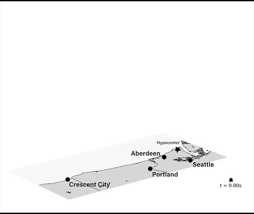
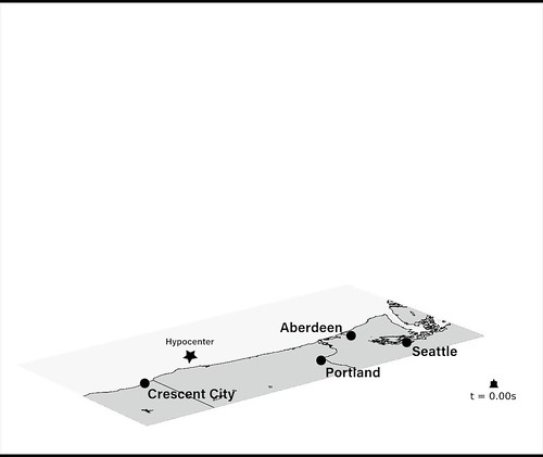
Out of an infinite number of possibilities, 50 simulations of an M9.0 earthquake were run by The M9 Project team. The individual earthquake scenarios had a few important variations between them, that made each earthquake source unique: (1) the hypocenter location (i.e., where the earthquake starts), (2) how far inland the rupture extends (i.e., how close the earthquake gets to major inland cities, such as Seattle), (3) the location of “sticky patches” on the fault, that generate the strongest ground shaking, and (4) the slip distribution on the fault (i.e., how far certain areas on the fault move during the earthquake).
Are certain earthquake scenarios “better” or “worse”?
The area affected by a megathrust earthquake is large enough that the outcome is going vary by location. A “best-case” scenario for one area in the Pacific Northwest could be a “worst-case” scenario somewhere else in the region.
One of the results of the computer simulations showed that when an M9.0 earthquake occurs on the Cascadia Subduction Zone, less violent shaking may be felt closer to the epicenter. This is because an earthquake on the Cascadia Subduction Zone will not occur at a single point -- instead, it will rupture a very large area. As the rupture moves along the fault, the seismic waves will start to “pile up,” similar to the Doppler Effect.

As the waves at the front of the rupture combine, their amplitudes get larger and create more violent ground motion. Therefore, locations closer to the hypocenter may receive less complex and destructive seismic waves than locations that are farther along the rupture and experience this “piling-up” of seismic energy.
In these two videos, notice how Seattle's mock seismogram has larger spikes (which denotes stronger ground motion) when the earthquake source is farther south, and the fault ruptures north.
This variation by location makes it virtually impossible to award a scenario the title “best-case” for the entire Pacific Northwest.
Can we do even better?
These computer simulations are the most accurate representations of what an M9.0 earthquake would look like in the Pacific Northwest. Unfortunately, there is a lot of variability in these calculations because there are still too many unknowns. An increase in seismic and GPS instrumentation throughout the Pacific Northwest, especially offshore, will help us identify more specifics about the Cascadia Subduction Zone and improve future computer simulations. For instance, we may be able to determine where “sticky patches” are located on the fault and obtain a more detailed image of the 3D structure of the subduction zone. Further constraining these variables in the computer simulations will ultimately help us refine our estimates of seismic hazards in the Pacific Northwest.
Special Thanks To
Dr. Erin Wirth, UW Affiliate Assistant Professor
M9 Simulation coverage from UW News
We are going to have The Big One. That’s a fact.
The final blog about The M9 Project is going to focus on you. What are you going to experience during a megathrust earthquake? How do we connect science and community? What should you do to be prepared?
The Next Stages of The M9 Project
Seismologists are not the only contributors to The M9 Project. Civil engineers, urban design and planners, statisticians, social scientists and public policy researchers also play a role in determining earthquake risk, safety measures, and public response to hazards.
Understanding the hazards and mechanisms of an earthquake is one thing, communicating effectively to the public is a completely different ball game. The next steps of The M9 Project focus on how we define and discuss hazards with communities.
For example, how does the way we design hazard maps affect how communities approach hazard planning? (See photo below) Or, how can hazards planning be steered towards rebuilding to community-specific values?

From assessing the utility of hazard maps (see image below), to hosting community planning workshops , The M9 Project’s research into “long term” preparedness- mitigation, response, and recovery focuses on how to best help you. We will discuss what to expect when the big one hits, as well as some resources so you can take steps to prepare .
Learning about Cascadia from other Large Earthquakes
The last megathrust earthquake on the Cascadia Subduction Zone occurred in 1700 AD, before written records were kept in the region. In addition to The M9 Project research at UW, we can also look to observations of other major earthquakes worldwide, to help us predict what The Big One may look like in the Pacific Northwest.
Ground Shaking
A magnitude 9 earthquake will generate very strong shaking for several minutes. The intensity, measured by the Modified Mercalli Intensity Scale (MMI), is determined by observations during an earthquake. Shaking tends to decrease farther away from the fault and will vary with local soil conditions, so intensity will vary by location. A more detailed description on intensity can be found here.
Below is a comparison of the shaking intensity from the 2001 Nisqually earthquake, compared to a hypothetical M9.0 earthquake scenario. A megathrust earthquake will be felt over a much larger area, and generate stronger shaking.


You can find more about how magnitude and intensity are related here.
As part of The M9 Project, UW civil engineers are researching building response to strong ground shaking from a magnitude 9.0 earthquake in Seattle. This video from Kinetica Dynamics shows skyscrapers in Tokyo shaking from the 2011 M9.0 Japan earthquake.
Tsunami
Large earthquakes on a subduction zone are capable of generating large tsunamis. For example, the 2004 M9.1 Sumatra earthquake resulted in a 30+ meter high tsunami on the west coast of Sumatra (source). For more about tsunamis, visit our tsunami overview page.
This NOAA video models the tsunami from the 1700 Cascadia earthquake, which caused damage and loss of life as close as the west coast of North America, and as far away as Japan.
We expect the next great Cascadia earthquake to be similar. As mentioned in our first M9 Project blog post, the record of past megathrust earthquakes can be found in muddy estuaries on the coast of the Pacific Northwest. In the layers of coast that have subsided and been filled again, there are bands of sand brought inland by tsunami waves, time and time again. Here is a article written by the American Museum of Natural History with more information on the Ghost Forests on the PNW.
Liquefaction
For liquefaction to occur, three things must happen. (1) Young, loose and grainy soil (2) needs to be saturated with water, and (3) experience strong ground shaking. The USGS, in coordination with California Geological Survey, give a summary of liquefaction and its effects here.
This video from the 2011 M9.0 Japan earthquake shows dramatic cracks in the ground, as well as liquefaction.
Our webpage on liquefaction includes video of the 2011 Christchurch earthquake, as well as links to liquefaction hazard maps for Washington and Oregon.
Landslides
Strong shaking can increase susceptibility to landslides.
This blog from the American Geophysical Union details some of the significant landslides in Paupa New Guniea that were triggered by a M7.5 earthquake on February 25th, 2011.
The Pacific Northwest is susceptible to landslides due to seasonal conditions, and strong shaking will increase landslide risk. Here are some resources from the states of Washington and Oregon.
Building Damage and Fires
The 1989 Loma Prieta earthquake caused widespread damage to infrastructure, such as the collapse of the Cypress Viaduct in Oakland, and fires in the San Francisco area.
Major cities in the Pacific Northwest would be just as susceptible to fire damage, and the construction of the Cypress Viaduct bears a striking resemblance to Seattle’s Alaskan Way Viaduct.


So, What Can I Do?
In order to prepare effectively, it is important to be aware of all earthquake-related hazards, such as the ones listed above. The following websites are great resources for earthquake hazards and preparedness in the Pacific Northwest. We encourage you to know your risks, be prepared, mitigate against hazards, respond safely, and enagae in holistic recovery planning.
- Cascadia Regional Earthquake Workgroup (CREW)
- Washington State Emergency Management Division
- State of Oregon Emergency Management
- Emergency Management British Columbia
- Become a Community Emergency Response Teams member
- Become a Red Cross Volunteer
- Check your local emergency management office for information specific to your community!
In the event of an earthquake, don't forget to drop, cover and hold!
Special Thanks To
Dr. Erin Wirth, Affiliate Professor, University of Washington
Lan T. Nguyen, Doctoral Student, Interdisciplinary Urban Design and Planning, University of Washington
On May 18th, 1980, at 8:32 AM, the landscape in Southwestern Washington was forever changed by an explosive eruption of Mount St. Helens. This was the most deadly volcanic event in US history.
Mount St. Helens is part of the Cascade Range, a chain of volcanoes from British Columbia to Northern California. The PNSN and the Cascades Volcano Observatory cooperatively operate 21 seismometers on or near Mount St. Helens, the most historically active volcano in the Cascade Range.

Seismogram of May 18th from one of our seismic stations.
Main PNSN Page on Mount St. Helens
Main CVO Page on Mount St. Helens
On the anniversary of the eruption of Mount St. Helens, earth science gets its day in the spotlight. Here's a collection of news stories about the eruption and what we have learned about volcanoes since 1980.
38 years later: What's changed since the Mount St. Helens Eruption?
- Q13 News
Features an interview with PNSN DIrector Emeritus Steve Malone
Mount St. Helens: Remembering the deadliest U.S. eruption 38 years later
- USA Today, King 5 News
Summary of events on May 18th, 1980 with photo galleries
Lessons Learned: Mount St. Helens to Kilauea
- King 5 News
Interview filmed in the PNSN Seismology Lab with Director Emeritus Steve Malone
Remembering Mt. St. Helens as Cascade event looms
- KOIN 6
Event overview, brief discussion of Cascade hazards, and dispels concern of a Kilauea-triggered event in the Cascades.
Photos: The Mt. St. Helens eruption of 1980
- KOIN 6
Includes an interview with CVO Scientist-In-Charge Seth Moran
Scientists Reflect on the Catastrophic 1980 Mount St. Helens Eruption
- Ashley Williams, AccuWeather
Details about the activity that led to the eruption, how life in the MSH area fared, and another Steve Malone feature.
How Dangerous are the Northwest's Volcanoes?
-KUOW, Oregon Public Broadcasting
Interview with CVO Scientist-In-Charge Seth Moran, discusses Oregon volcano hazards
Background: The Challenges of Predicting Seismic Hazard
We all want to know when the next big earthquake will happen. But because we can’t predict earthquakes, the next best thing we can do is figure out how strong shaking could be during future quakes. To do this, earth scientists can reconstruct an area’s historic earthquake record using geologic markers and any available written accounts, which allows them to constrain recurrence and magnitude ranges for quakes on local faults. Scientists then combine these estimates with what we know about an area’s surface geology to predict how often and how strong the ground will shake during an earthquake. This sort of analysis is the basis for the US’ National Seismic Hazard Mapping Project, and it is critical for making sure we build structures that can withstand earthquake shaking.
Predicting how an earthquake will shake an area is not a trivial task, however. Besides the challenges of figuring out the historical earthquake record from sparse geologic markers, understanding how conditions at a given location will affect earthquake shaking is very difficult. In Seattle, for example, there are many interesting geologic features that change and amplify ground motion during earthquakes; large areas of water-logged, artificial fill under Pioneer Square and SODO have amplified ground motion and even liquefied during historic earthquakes; the deep Seattle Basin, which contains thick layers of relatively soft sediments, traps seismic waves and “sloshes” like a big bowl of jelly in some earthquakes. Taking these effects into consideration during seismic hazard analysis is important, but requires a detailed understanding of the local geology and how it affects seismic waves.
The hills are alive with the sound of … earthquakes?
A geographic component that is not often considered during seismic hazard analysis is topography. As seismic waves from an earthquake propagate through the earth, they interact with subsurface geology, like faults and basins; however, the waves also interact with surface features, like hills, cliffs, and valleys. Depending on the wavelength of the seismic waves and the direction they’re traveling, the shaking felt on these features can be much stronger (or weaker!) than in surrounding flat areas. This amplification happens because these features scatter and trap seismic energy; they can also experience a sort of structural “resonance”, similar to the way buildings and bridges can. Studies of ground motion from the 2009 L’Aquila and 2010 Haiti earthquakes [1, 2] have shown that topography significantly amplified ground motion at certain locations, sometimes shaking twice as strong as surrounding areas!
With these findings in mind, we are interested in seeing how topography might affect earthquake shaking here in Seattle. While the city doesn’t have any particularly tall or prominent ridges, it does have many steep bluffs and cliffs overlooking Elliott Bay and Puget Sound. We know from past earthquakes that these features are prone to land-sliding, and we would like to know how topographic amplification might contribute to that hazard, as well as to the general safety of structures built on the bluffs.
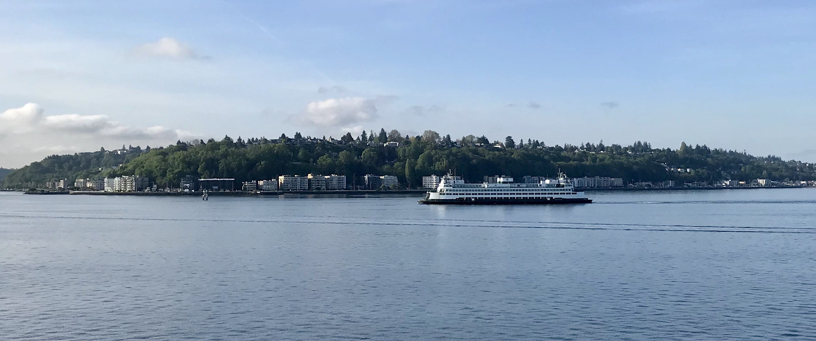
How will the 70-90m tall bluffs around the city behave in an earthquake?
How will things shake out in West Seattle?
So, as part of a graduate-student-led research project, we are looking for volunteers in West Seattle to host seismometers for a small experiment. In this project, portable seismometers will be placed along and down the bluffs facing Puget Sound. Over the course of a few hours, these seismometers will record the ambient vibrations caused by ocean waves, weather systems, and even car traffic. Together, these sources create what’s known as ambient seismic noise. By comparing recordings of this noise from points along the bluff, we can understand how the topography amplifies ground shaking during earthquakes.
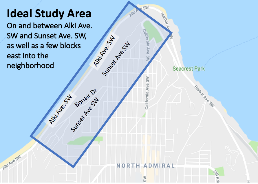
For our experiment, we are looking for hosts in West Seattle living near the bluffs along Alki. Ideally, hosts would live on or between Sunset Ave. SW and Alki Ave. SW. We also need a few sites in the neighborhood away from the sea bluff (see the map below). The experiment itself will last just 1 day, and only requires access to your yard, where we will plop-down a coffee-can sized seismometer for a few hours. The experiment will take place some time between early October and late November.
So, if you are a citizen scientist who would like to help us better understand how earthquakes rattle the hills around our city, and you live on or near the Sound-facing bluffs in West Seattle, please consider filling out the form linked below!
If you have any questions about the experiment, you can contact the project lead Ian Stone at ipstone@uw.edu
Link to Sign-up Form: https://forms.gle/vfSBgpZUapbKs5eo7
References
[1] Massa, M., Lovati, S., D’Alema, E., Ferretti, G., and M. Bakavoli, 2010. An experimental approach for estimating seismic amplification effects at the top of a ridge, and the implication for ground-motion predictions: The case of Narni, Central Italy. Bul. Seis. Soc. Amer., 100 (6) 3020-3034.
[2] Hough, S. E., Altidor, J. R., Anglade, D., Given, D., Janvier, M. G., Maharrey, J. Z., Meremonte, M., Mildor, B. S. L., Prepetit, C., and A. Yong, 2010. Localized damage caused by topographic amplification during the 2010 M 7.0 Haiti earthquake. Nature Geoscience, 3. 778-782.